Gradient Reduction Part 1 (AutomaticBackgroundExtractor)
At this point in the tutorial, you have learned a few key skills:
You have also learned a bunch of more general PixInsight skills such as the use of preview areas, using Real-Time Previews, and saving process icons.
It is time to add another key skill to your inventory, gradient reduction. Unless you shoot under perfectly dark skies, have perfect calibration data (such as flats), and the Moon isn't up, you have gradients in your image. Those gradients are of three main types:
A gradient is simply a change in light across the image that is not due to your target. Lets talk about each of these three types. Gradients caused by imperfect calibration show up a number of ways. For example it is common for a flat to not perfectly correct the vignetting of an image. The middle portion of the image may be too dark or too light compared to the corners. Or you may have a situation where a vertical or horizontal band shows up in the image because of imperfect flats, darks, or bias.
An example of a gradient caused by an unwanted signal is one due to light pollution or the Moon. In this case it is common for the image to be slightly brighter in the parts closest to the Moon or closest to the brightest part of the light pollution. And likewise, the areas furthest from the Moon or the brightest parts of the light pollution will be darker. So you have a gradual change from a light area on one side of the image to a darker area on the other side of the image.
A common example of differential atmospheric dispersion is seen when the Sun is setting. The reds are dispersed less than the blues, and so the Sun appears orange.
Let me state up front that many gradient problems that people attribute to light pollution or the Moon or some other signal are in fact due to imperfect calibration or atmospheric dispersion. Also, all three kinds of gradient can be complicated by Meridian flips where the gradient was one direction on one side of the flip and another after the flip. The two results on the two sides of the flip get averaged together and you can get things like two bright diagonal corners and a darker stripe between the other two diagonal corners.
Gradients show up in almost every image, and are bad enough to benefit from some correction in most images. They are particularly easy to see in the color data.
At this point in the tutorial, you have learned a few key skills:
- The Use of the ScreenTransferFunction
- Using DynamicCrop to crop out stacking artifacts
- How to stretch your image using a variety of tools
- How to use CurvesTransformation to increase contrast in parts of the image
You have also learned a bunch of more general PixInsight skills such as the use of preview areas, using Real-Time Previews, and saving process icons.
It is time to add another key skill to your inventory, gradient reduction. Unless you shoot under perfectly dark skies, have perfect calibration data (such as flats), and the Moon isn't up, you have gradients in your image. Those gradients are of three main types:
- Those caused by imperfect calibration
- Those cause by an unwanted signal
- Those caused by differential atmospheric dispersion
A gradient is simply a change in light across the image that is not due to your target. Lets talk about each of these three types. Gradients caused by imperfect calibration show up a number of ways. For example it is common for a flat to not perfectly correct the vignetting of an image. The middle portion of the image may be too dark or too light compared to the corners. Or you may have a situation where a vertical or horizontal band shows up in the image because of imperfect flats, darks, or bias.
An example of a gradient caused by an unwanted signal is one due to light pollution or the Moon. In this case it is common for the image to be slightly brighter in the parts closest to the Moon or closest to the brightest part of the light pollution. And likewise, the areas furthest from the Moon or the brightest parts of the light pollution will be darker. So you have a gradual change from a light area on one side of the image to a darker area on the other side of the image.
A common example of differential atmospheric dispersion is seen when the Sun is setting. The reds are dispersed less than the blues, and so the Sun appears orange.
Let me state up front that many gradient problems that people attribute to light pollution or the Moon or some other signal are in fact due to imperfect calibration or atmospheric dispersion. Also, all three kinds of gradient can be complicated by Meridian flips where the gradient was one direction on one side of the flip and another after the flip. The two results on the two sides of the flip get averaged together and you can get things like two bright diagonal corners and a darker stripe between the other two diagonal corners.
Gradients show up in almost every image, and are bad enough to benefit from some correction in most images. They are particularly easy to see in the color data.
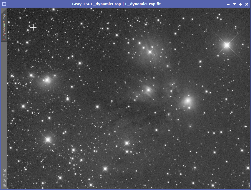
Cropped Luminosity Data with STF and Gradients Still Uncorrected
The image above shows my cropped luminosity data with a STF (ScreenTransferFunction) and the gradients still uncorrected. My experienced eye can spot where I think there are some gradients, but a less experienced eye might assume there aren't any.
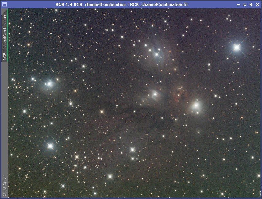
Cropped Color Data with STF and Uncorrected Gradients
We haven't gone into working with color data yet, but in the above image, notice how much easier it is to see gradients in the color data. For example the four corners of the image have very different colors and some corners appear brighter than the others as well. For example the upper left corner looks pretty dark compared to the others.
In PixInsight, there are two main tools that are used to deal with gradients:
In general, the DynamicBackgroundExtraction tool is more capable but also more difficult to use and understand. We will start with the AutomaticBackgroundExtractor process. My advice would be that until you get really familiar and comfortable with the DynamicBackgroundExtraction (DBE) process, try the AutomaticBackgroundExtractor (ABE) first. If it does the job, good enough and move on.
So how does AutomaticBackgroundExtractor Work? Basically, it makes sample boxes throughout the image. It looks at the intensity of the light in those samples, and tries to fit a curve to those samples that describe the gradient. In places where there are bright structures like nebulae, stars, or galaxies, the sample box may be skipped since we are really only interested in the unwanted signal that makes up a gradient. Rejection parameters control whether a box will be sampled or not.
In PixInsight, there are two main tools that are used to deal with gradients:
- AutomaticBackgroundExtractor
- DynamicBackgroundExtraction
In general, the DynamicBackgroundExtraction tool is more capable but also more difficult to use and understand. We will start with the AutomaticBackgroundExtractor process. My advice would be that until you get really familiar and comfortable with the DynamicBackgroundExtraction (DBE) process, try the AutomaticBackgroundExtractor (ABE) first. If it does the job, good enough and move on.
So how does AutomaticBackgroundExtractor Work? Basically, it makes sample boxes throughout the image. It looks at the intensity of the light in those samples, and tries to fit a curve to those samples that describe the gradient. In places where there are bright structures like nebulae, stars, or galaxies, the sample box may be skipped since we are really only interested in the unwanted signal that makes up a gradient. Rejection parameters control whether a box will be sampled or not.
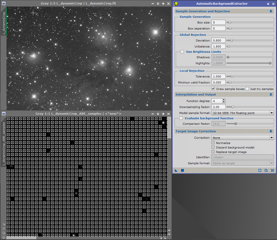
Luminosity Data with AutoMaticBackgroundExtractor (ABE) Interface and the Sample Boxes
In the above image I show the default ABE settings and the sample boxes that that default creates for the cropped unstretched luminosity data (shown with a STF). Usually, you want to do Gradient reduction on the linear (unstretched) data. I forced ABE to actually show the sample boxes by checking the "Draw Sample Boxes" check box (the one non default setting above). Notice the sample boxes were not drawn around some of the stars. If I panned the view, you would see that they were not created around some of the nebulosity as well.
Normally the defaults for Box Size, Box Separation, and the various Global Rejection and Local Rejection parameters work reasonably well.
By reducing the Global Deviation Parameter you can exclude more sample boxes around stars and the nebulae. Likewise, increasing it will allow sampling more of the large scale structures (something you normally don't want). Although the default tends to work reasonably well, this is a parameter you may occasionally want to try varying.
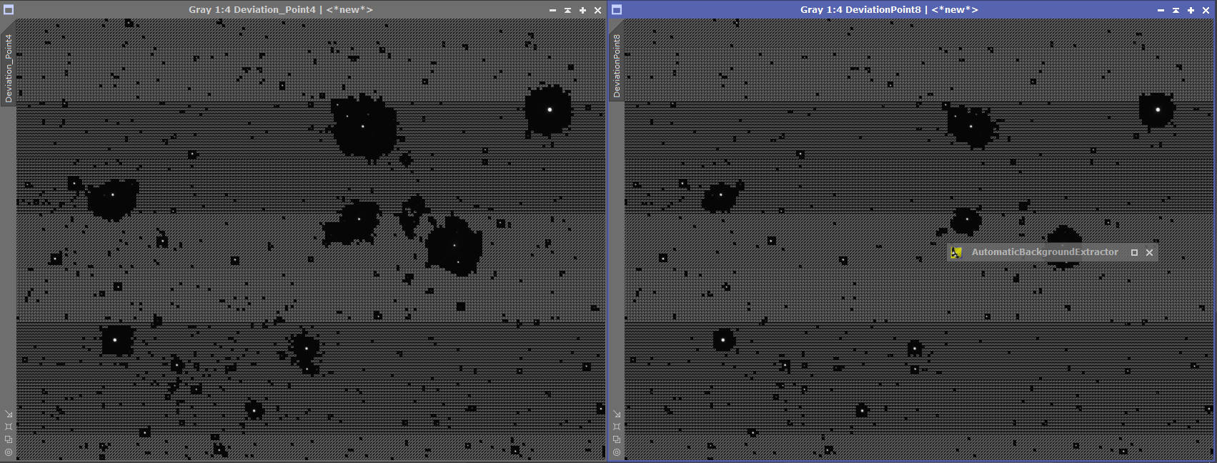
A Comparison of Global Rejection Deviation .4 (left) vs .8 (Right)
In the image above is a comparison where the Global Rejection Deviation parameter was changed to .4 (left) from the default .8 (right). More sample boxes have been excluded at the .4 setting.
In my experimentation the Unbalance parameter under global rejection rarely makes much difference. Likewise, in practice, I have not found the Use Brightness Limits section of the Global Rejection parameters to be much value. You can easily make the shadow parameter too large where it will not create any sample boxes at all, and the before that point, the slider is not very sensitive.
The Local Rejection Parameters DO make a difference but there is not a good visual feedback mechanism, so I suggest that in practice you leave them alone. Fortunately the defaults are normally reasonable. There is an equivalent in DynamicBackgroundExtractor (DBE) that is more useful in practice. To explain what they are doing, in each sample box there are pixels with different values. The Local Rejection parameters control what is considered an outlier in a sample box. Outliers are not used to calculate the intensity value of the sample box as a whole.
Next we come to a section of the ABE Interface that is CRUCIAL to getting good results, Interpolation and Output. And unfortunately the Interpolation and Output portion of the interface is not expanded when you first bring up ABE. The same is true of the Target Image Correction section. And without making some changes to the Target Image Correction section, the ABE won't even fix your gradients! I really don't understand why the authors of PixInsight made certain choices. [Shaking my head].
So lets do an ABE on the dynamically cropped luminosity data. Here is what the gradient detected looks like at Function degree 0.
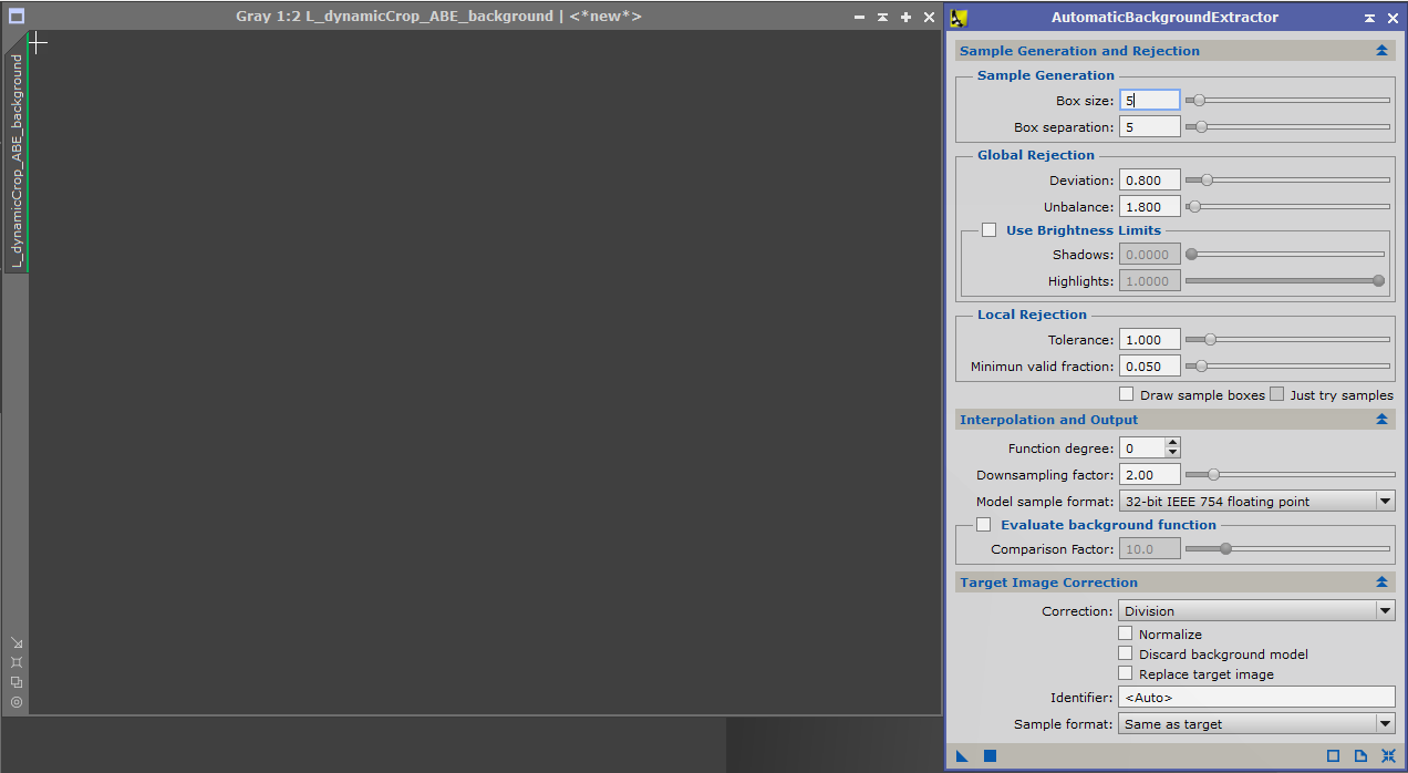
Gradient Found by ABE at Function Degree 0
Well at first glance, that doesn't look like a very interesting result. Basically it is the average intensity of all those sample boxes over the entire image. It doesn't vary at all. For the more mathematically inclined a 2D polynomial expression of function degree 0 has been used to fit the intensity found in the sample boxes.
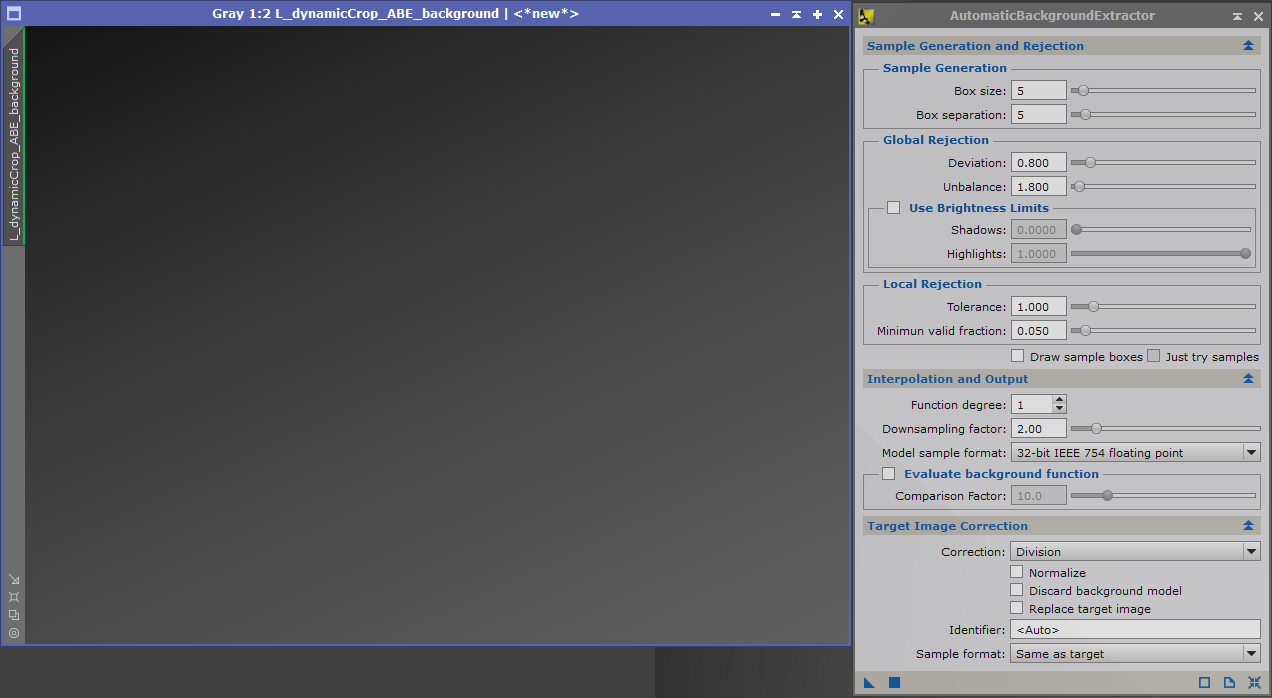
Gradient Found by ABE at Function Degree 1
Now what happens if Function degree 1 is used. In that case a linear fit is made to the data in both the X and Y directions so we intensities varying in linear way on both the X and Y axis.
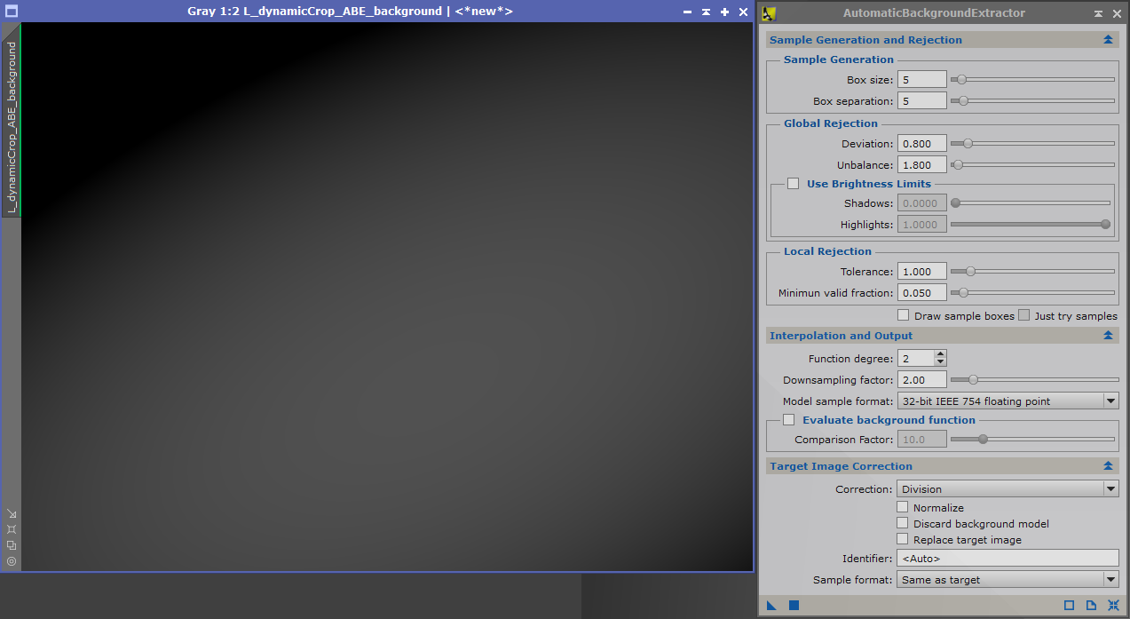
Gradient Found by ABE at Function Degree 2
By the time we get to Function degree 2, things are getting quite a bit more complex. For the mathematically inclined now a 2nd degree polynomial has been fitted to the data from the sample boxes. For example in the x direction a polynomial of the form Ax**2 + Bx +C has been fitted to the data. The same is true in the y direction.
Each time we increase the Function degree we are using more and more complicated polynomials (ones with more terms) to fit the data.
Gradients are usually not very complicated things. They tend to vary smoothly and slowly over an image. If a high function degree is used to fit the sample boxes, you stand a very real risk of over fitting the data and eliminating structure that was really there. As a rule of thumb, you should start at Function Degree 1 and use the lowest function degree that eliminates the gradients that are clearly not target signal. This will often be Function Degree 1 or 2. The default value of 4 is often much more complicated than is actually necessary and does harm to your image. I put that in bold because it is important. I have found images that required Function degree 4, but don't start there. Again, use the minimum function degree necessary to correct the gradient.
On to the Target Image Correction portion of the interface. Unless you set a correction action with the Correction drop down, the gradient found will not actually be removed from the image. There are two choices:
The proper one to use can (and has) generated all kinds of arguments. If you look at the tool tips, they suggest the following:
There are those who believe that many of the problems normally thought to be caused by light pollution or the Moon are actually calibration problems or differential atmospheric dispersion (recall the setting Sun example I gave earlier). As such they recommend using Division as your default. Others believe the issue commonly is light pollution or the Moon and they recommend using subtraction.
Now for the pragmatist view. In my experience, it rarely makes much difference, and when it does make a difference, I found that division often gives a slightly (and I do mean slightly) less noisy result.
I tend to use division by default. Your mileage may vary (YMMV), And I recognize many other tutorials/books will recommend subtraction as the default.
Back to the tutorial image. Let us try Division and at Function degree 1 and 2.
Each time we increase the Function degree we are using more and more complicated polynomials (ones with more terms) to fit the data.
Gradients are usually not very complicated things. They tend to vary smoothly and slowly over an image. If a high function degree is used to fit the sample boxes, you stand a very real risk of over fitting the data and eliminating structure that was really there. As a rule of thumb, you should start at Function Degree 1 and use the lowest function degree that eliminates the gradients that are clearly not target signal. This will often be Function Degree 1 or 2. The default value of 4 is often much more complicated than is actually necessary and does harm to your image. I put that in bold because it is important. I have found images that required Function degree 4, but don't start there. Again, use the minimum function degree necessary to correct the gradient.
On to the Target Image Correction portion of the interface. Unless you set a correction action with the Correction drop down, the gradient found will not actually be removed from the image. There are two choices:
- Subtraction
- Division
The proper one to use can (and has) generated all kinds of arguments. If you look at the tool tips, they suggest the following:
- Use Subtraction when the gradient is caused by unwanted signal such as the Moon or Light Pollution
- Use Division when the problem is caused by things like flats not quite properly correcting (vignetting) or differential atmospheric dispersion (light being scattered differentially by the atmosphere).
There are those who believe that many of the problems normally thought to be caused by light pollution or the Moon are actually calibration problems or differential atmospheric dispersion (recall the setting Sun example I gave earlier). As such they recommend using Division as your default. Others believe the issue commonly is light pollution or the Moon and they recommend using subtraction.
Now for the pragmatist view. In my experience, it rarely makes much difference, and when it does make a difference, I found that division often gives a slightly (and I do mean slightly) less noisy result.
I tend to use division by default. Your mileage may vary (YMMV), And I recognize many other tutorials/books will recommend subtraction as the default.
Back to the tutorial image. Let us try Division and at Function degree 1 and 2.
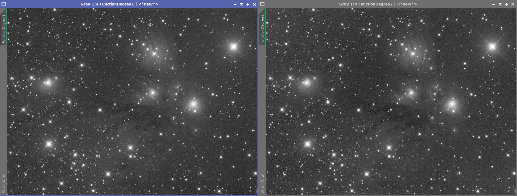
ABE at Function Degree 1 (Left) and 2 (Right) with Division
The differences between Function Degree 1 and 2 are subtle but real. And part of getting good at image processing is noticing the subtle. In general the corners of the Function Degree 1 image are less well corrected. The left upper corner is still significantly darker than the others. The right upper corner has a drop in light towards the very corner that is not likely to be real. Furthermore, the dark nebulae strands in the middle of the image are more distinct in the image using Function Degree 2.
I could have tried higher Function Degrees but it is my judgement that the image at Function Degree 2 is already well corrected, and that would be the image I would use. Again, as a rule, use the lowest Function degree that gets the job done.
I could have tried higher Function Degrees but it is my judgement that the image at Function Degree 2 is already well corrected, and that would be the image I would use. Again, as a rule, use the lowest Function degree that gets the job done.
